🦾

Dueling DQN

생성일

2024/07/22 03:00

최종 수정일

2025/11/11 06:46

태그

강화학습

작성자

1. Introduction

•

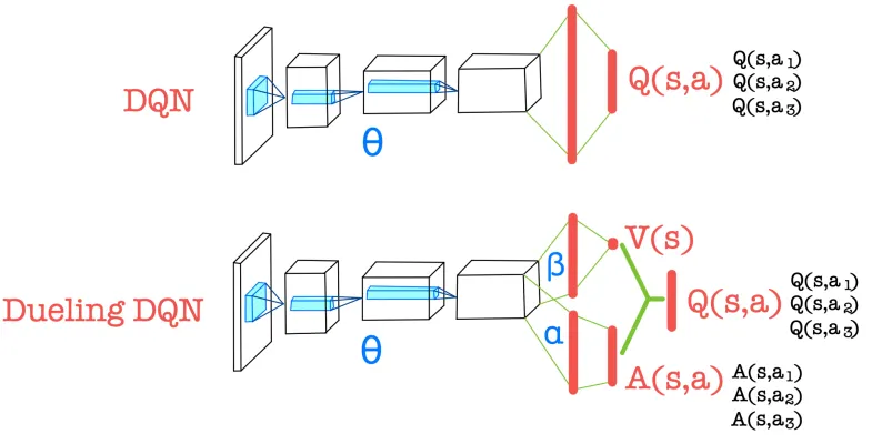
Compute the advantage function and the state-value function separately, then combine them to obtain the action-value function.

•

The CNN encoder is shared, while only the parameters of the fully connected layers differ for each function.

•

Useful for evaluating the state value even when the action is not significant in the environment.

2. Value function

•

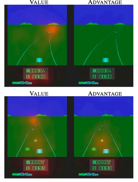
When actions have little influence on the environment in a given state, learning V(s)V(s)V(s) becomes more important for accurately evaluating the state value.

•

When actions have little influence on the environment in a given state, learning V(s)V(s)V(s) becomes more important for accurately evaluating the state value.

•

First case (the car is at a distant position)

◦

The importance of action selection decreases.

◦

Only when computing the state value, the car in front is considered.

•

Second case (the car is at a close position)

◦

The choice of action becomes more important.

◦

Each nearby car is also taken into account when computing the advantage.

3. Identifiability issue

•

The relationship among the Action value function, Advantage function, State value function

{\small \quad Q^{\pi}(s, a) = V^{\pi}(s) + A^{\pi}(s, a)}

{\small \quad \mathbb{E}_{a \sim \pi(s)} [ Q^{\pi}(s, a) ] = V^{\pi}(s) \quad \Rightarrow \quad\mathbb{E}_{a \sim \pi(s)} [ A^{\pi}(s, a) ] = 0}

{\small \quad a^* = \arg\max_a Q(s, a')}

{\small \therefore \quad Q^*(s, a^*) = V^*(s) \quad \Rightarrow \quad A^*(s, a^*) = 0}

•

In Dueling DQN separate networks are used to compute the state-value function and the advantage function.

◦

The decomposition of a single Q-value is not uniquely defined.

▪

 (V(s)+const)+(A(s,a)−const)(V(s)+const) + (A(s,a) -const)(V(s)+const)+(A(s,a)−const)

▪

V(s;θ,β)V(s ; \theta, \beta)V(s;θ,β), A(s,a;θ,α)A(s,a ; \theta, \alpha)A(s,a;θ,α) can’t be regarded as a good estimator.

•

Approach 1) Add an advantage function term for the optimal action.

◦

For the optimal action, the following property holds.

{\small \quad Q^*(s, a^*) = V^*(s) \quad \Rightarrow \quad A^*(s, a^*) = 0}

◦

Q(s,a∣θ,α,β)=V(s∣θ,β)+[A(s,a∣θ,α)−max⁡a′A(s,a′∣θ,α)]{\small Q(s, a \mid \theta, \alpha, \beta) = V(s \mid \theta, \beta)+ \left[ A(s, a \mid \theta, \alpha) - \max_{a'} A(s, a' \mid \theta, \alpha) \right]}Q(s,a∣θ,α,β)=V(s∣θ,β)+[A(s,a∣θ,α)−maxa′​A(s,a′∣θ,α)]
⇒a∗=arg⁡max⁡a′Q(s,a′∣θ,α,β)thenmax⁡a′A(s,a′∣θ,α)=A(s,a∗∣θ,α){\small \Rightarrow  a^* = \arg\max_{a'} Q(s, a' \mid \theta, \alpha, \beta)
\quad \text{then} \\ \quad
\max_{a'} A(s, a' \mid \theta, \alpha) = A(s, a^* \mid \theta, \alpha)}⇒a∗=argmaxa′​Q(s,a′∣θ,α,β)thenmaxa′​A(s,a′∣θ,α)=A(s,a∗∣θ,α)

◦

Since the max term has high variability, it reduces stability.

•

Approach2) Subtract the mean

◦

Q(s,a∣θ,α,β)=V(s∣θ,β)+[A(s,a∣θ,α)−1∣A∣∑a′A(s,a′∣θ,α)]{\small Q(s, a \mid \theta, \alpha, \beta)= V(s \mid \theta, \beta)+\left[ A(s, a \mid \theta, \alpha)-\frac{1}{|\mathcal{A}|} \sum_{a'} A(s, a' \mid \theta, \alpha) \right]}Q(s,a∣θ,α,β)=V(s∣θ,β)+[A(s,a∣θ,α)−∣A∣1​∑a′​A(s,a′∣θ,α)]

◦

For the optimal action, an error equal to the difference between the max and the mean occurs.

▪

The objective is to find the action that maximizes QQQ 

▪

This is equivalent to maximizing the term composed of the advantage function.

▪

Whether the max or the mean is subtracted does not affect policy determination.

▪

This is because the state-value function does not vary with the action.