1. Introduction
•
Introduced a CNN architecture to handle high-dimensional image inputs
◦
Enables processing of high-dimensional and continuous state spaces
•
Represents Q-values through a Q-network
◦
Since Q-values must be output for all actions, the action space must be discrete, finite, and of much lower dimensionality compared to the state space
2. DQN Architecture
•
Input
◦
To satisfy the Markov property, four consecutive frames are stacked as the input.
◦
A single frame does not contain sufficient information to predict the future in terms of velocity and direction.
◦
Since the Q-value is computed for a given state input, there are few constraints on the dimensionality of the state space.
•
Convolution Layer
◦
Applies convolution operations to the input images to extract feature vectors and reduce dimensionality.
◦
The last feature maps are flattened so that they can be processed by fully connected layers.
◦
Because spatial information is crucial in games, max pooling—which tends to blur positional details—is not applied.
•
Output
◦
Produces Q-values for each possible action.
◦
The network parameters are updated to ensure that the predicted Q-values approximate the optimal Q-values.
3. Naive DQN
•
Q-learning
◦
Target policy: A greedy policy w.r.t
◦
Behavior policy: An w.r.t
◦
The learning process updates the network in a way that minimizes the difference between the Q-value of the current state and its target value.
•
Naive DQN
◦
Define the loss function as the Mean Squared Error
◦
The network is updated by minimizing it
•
Problems
◦
Temporal Correlations
▪
In online RL, parameter updates are executed based on transitions collected over time.
▪
Strong correlations exist between consecutive transitions, which can lead the network to overfit to specific situations.
▪
As a result, the model may fail to sufficiently learn from rare but important experiences.
◦
Non-stationary target
▪
Since the same Q-network is used both to compute the target and to update the Q-values, the target function changes frequently, making convergence difficult.
4. Replay buffer
•
Addressing the Temporal Correlation problem
•
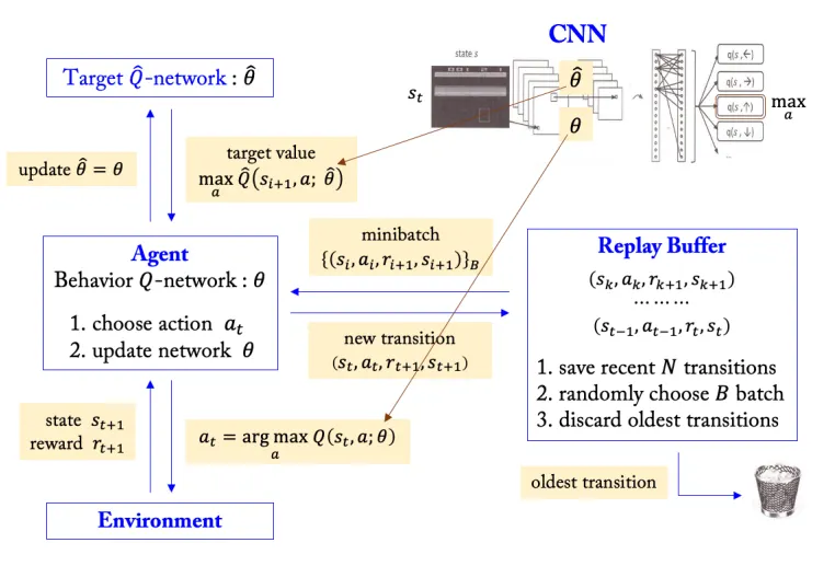
Store transitions in replay buffer and randomly sample minibatches from it for training
•
This reduces temporal correlations between transitions, as each batch can be composed of experiences from different experience and time steps.
•
Improve training efficiency
•
Past experiences can be reused
5. Target Network
•
Initialize the target Q-network parameters to be identical to the behavior Q-network parameters at the start of training.
•
During training, fixed while continuously updating .
•
After a certain number of steps, update by copying .
•
This approach stabilizes training by addressing the problem of a continuously changing target function.
6. DQN
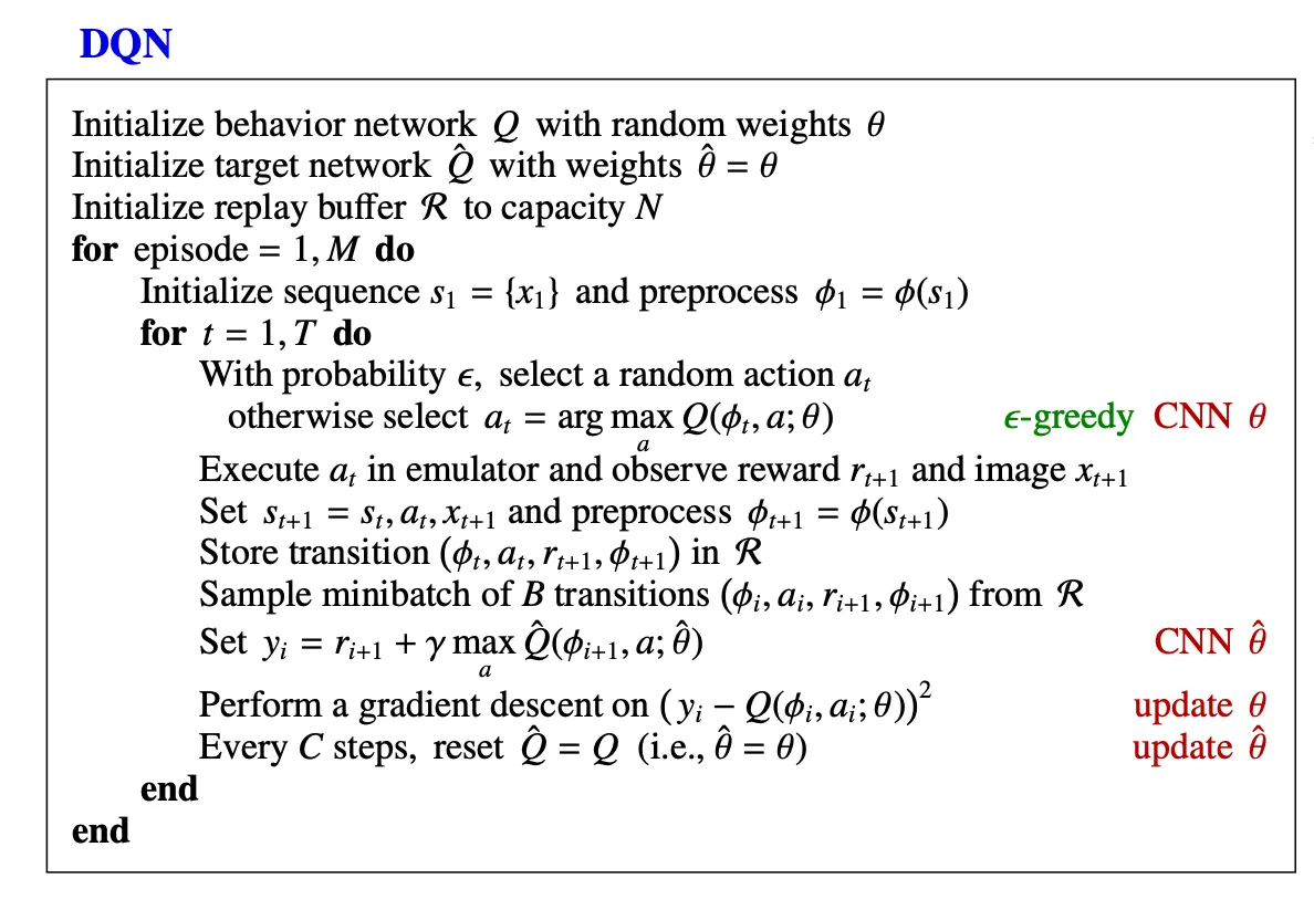
1.
From the current state , select an action using the policy based on the behavior network parameters.
2.
Store the transition in the replay buffer.
3.
The replay buffer holds the most recent transitions; when a new transition is added, the oldest one is removed.
4.
Randomly sample a minibatch of transitions from the replay buffer.
5.
For the sampled data, compute the target values using the target network parameters.
6.
Compute the loss function .
•
•
7.
Update the behavior network parameters.
8.
After a fixed number of steps, update the target network parameters.
7. Multi-step Learning
Multi-step learning refers to training that uses the n-step return when computing the target values. By choosing an appropriate number of steps, the learning speed can be improved. The loss function used in multi-step learning is defined as follows.
•
•


